Using Timescale's Continuous Aggregates to speed up database queries
Table of Contents
Introduction #
During my internship at Magenta, that helped me finish my master’s thesis in Computer Science & Engineering at UNIFI, I was tasked with improving the performance of some very specific database queries for the AirQino platform (also check out previous post on implementing PostgreSQL’s streaming replication).
The problem #
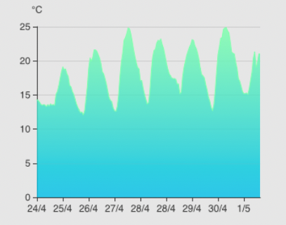
One of the main features of the AirQino platform is showing trends of different air quality factors (such as temperature, humidity, CO2, NO2, PM2.5, PM10, O3 etc…) in the last seven days of measurements, in the form of a simple chart like this:

In order to show this, all data of the past week must be extracted and then aggregated into hourly averages. This was done using a SQL query similar to this, leveraging Timescale’s useful time_bucket function:
1SELECT time_bucket('1 hour', sd.data_acquired) as bucket, avg(sd.float_value) FROM station_data sd2WHERE sd.data_acquired > NOW() − INTERVAL '7 days'3AND sd.sensor_id = XXX4ORDER BY bucket DESC;Where station_data is the table containing the sensor data, data_acquired column represents the measurement date and time, and the float_value column indicates the raw value of the measurement. The data is limited only to the last week through a WHERE clause.
However, this means that if you want to run this query more than once, the database must scan the entire table and recalculate the average each time. This is inefficient, because in most cases the data in the table has not changed significantly, so there is no need to scan it again.
Here are the query response times to extract the hourly average of NO2 for all AirQino stations, before applying the optimization:

As we can see performance is not great (even over 30 seconds!) for stations having with the most data points.
To improve this and make data aggregation faster, Timescale provides a feature called continuous aggregates.
Continuous Aggregates #
From the official documentation:
TimescaleDB continuous aggregates use PostgreSQL materialized views to continuously and incrementally refresh a query in the background, so that when you run the query, only the data that has changed needs to be computed, not the entire dataset.
Here are the steps required to implement it:
- A hypertable was created starting from the original table, taking care to migrate all the data (this is necessary because continuous aggregates only apply to hypertables), using the command:
SELECT create_hypertable('station_data', 'data_acquired', migrate_data => true);Where data_acquired is the time column of the table, where the measurement date and time are saved. This operation may take a long time depending on the amount of data in the table: on the AirQino production database it took about 36 minutes.
- Then, create a materialized view for calculating hourly averages with continuous aggregates:
1CREATE MATERIALIZED VIEW station_data_hourly_avg WITH (timescaledb.continuous) AS2SELECT time_bucket('1 hour', sd.data_acquired) AS bucket, station_id, sensor_id, avg(sd.float_value)3FROM station_data sd4GROUP by bucket, station_id, sensor_id;Where the name of the aggregate is station_data_hourly_avg, while the continuous aggregation functionality is specified in the WITH clause. In the SELECT, on the other hand, the starting table (station_data), the aggregation interval (1 hour) and the operation to be performed to aggregate the data (avg(), the average) were specified. This operation on the AirQino production database took about 5 minutes.
- Finally, create a refresh policy with:
1SELECT add_continuous_aggregate_policy('station_data_hourly_avg',2 start_offset => INTERVAL '7 days',3 end_offset => INTERVAL '1 hour',4 schedule_interval => INTERVAL '1 hour'5);Where start_offset indicates how far back in time the aggregate is calculated, end_offset indicates when to stop and schedule_interval indicates the view update interval. Here we chose to update the data of the past week every hour, up to one hour before the execution time. For performance reasons, it is always advisable to exclude the last bucket (in this case the last hour of data arrived).
Results #
Once the continuous aggregate view is up and running, we can rewrite the original query:
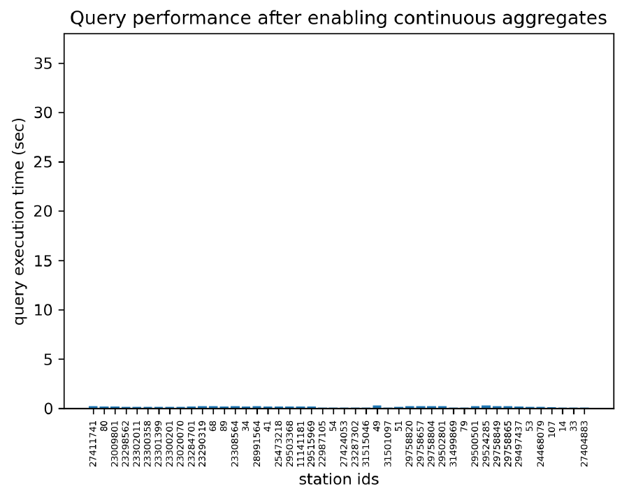
1SELECT sd.avg2FROM station_data_hourly_avg sd3WHERE sd.bucket > NOW() − INTERVAL '7 days'4AND sd.sensor_id = XXX ORDER BY sd.bucket DESC;Since the hourly averages are now pre-calculated and always updated in the background, this query has much faster response times:

Using the new query, optimized with continuous aggregates, the response times are constant for all stations, regardless of the amount of data. This improvement has led to a significant reduction in response times, now in the order of milliseconds, ensuring greater scalability and efficiency to the system.
Conclusion #
Timescale’s continuous aggregates feature is a great way to take raw data from a table, aggregate it, and store the intermediate state in a materialization hypertable that is always updated in the background. The addition of configurable refresh policies gives you full control over how much data is aggregated and how frequently it is updated.
Check out the official documentation for more information!